FishDiveR tutorial

The full workflow, step by step: from a raw tag archive to days grouped into behaviour clusters. It uses the example tag that comes with the package, and every figure on this page is real FishDiveR output.

This tutorial follows the development version of FishDiveR (1.1.0.9000) on GitHub. A few options it uses, such as minmax_bins for fast plotting, are not yet in the CRAN release (1.1.0). Prefer not to write code? The same workflow runs in the point-and-click app.

How the method works

The unit of analysis is the day: each 24-hour period, midnight to midnight in local time, becomes one row of data to cluster.

Wavelet analysis. A continuous wavelet transform finds how strongly the depth record oscillates at each period (for example every 20 minutes, every 3 hours, once a day) at every point in time. Unlike a Fourier transform, it copes with behaviour that changes through the record.
Daily statistics. The wavelet results are summarised for each day and each period (mean power, power variance, mean amplitude and so on). Separately, daily depth statistics are calculated from the depth record itself: mean and maximum depth, vertical speed, time near the surface and, optionally, differences between day and night.
Principal component analysis (PCA). Neighbouring wavelet periods carry very similar information, so the many wavelet statistics are condensed into a few principal components.
K-means clustering. The principal components and depth statistics are combined, and the days are grouped into k clusters of similar behaviour.

The method is described in detail in the methods paper: Beale et al. (2026), Movement Ecology 14, 8, doi.org/10.1186/s40462-025-00622-w.

Install and set up

# install.packages("remotes")
remotes::install_github("calvinsbeale/FishDiveR", build_vignettes = TRUE)

Every step saves its results in a project folder, with one sub-folder per tag (and a Combined_tags folder when several tags are analysed together). Later steps read the earlier results from there. This example uses a temporary folder; for your own data, use a permanent one.

# Use rgl's off-screen device, as k_clustering() can draw a 3D plot
options(rgl.useNULL = TRUE)
library(FishDiveR)

# Example data shipped with the package
example_folder <- system.file("extdata", package = "FishDiveR")

# Project folder for the results
project <- file.path(tempdir(), "FishDiveR-vignette")
dir.create(project, showWarnings = FALSE)

1. Import the depth record

import_tag_data() reads a CSV archive with a date-time column and a depth column, crops it to the deployment, and then to whole days (midnight to midnight) in the local time zone. The cropped record is saved as archive_days.rds in the tag’s folder.

archive_days <- import_tag_data(
  tag_ID = "data",
  tag_deploy_UTC = "2000-01-01 00:00:00",
  tag_release_UTC = "2000-01-11 23:59:00",
  archive = file.path(example_folder, "data", "data-Archive.csv"),
  date_time_col = 1,
  depth_col = 2,
  time_zone = "UTC",
  output = TRUE,
  output_folder = project
)
head(archive_days)
#>                   date depth  date_only
#>                 <POSc> <num>     <Date>
#> 1: 2000-01-01 00:00:00  13.9 2000-01-01
#> 2: 2000-01-01 00:01:00  10.8 2000-01-01
#> 3: 2000-01-01 00:02:00  16.5 2000-01-01
#> 4: 2000-01-01 00:03:00  14.8 2000-01-01
#> 5: 2000-01-01 00:04:00   4.7 2000-01-01
#> 6: 2000-01-01 00:05:00  12.1 2000-01-01

Three things to check with your own data:

Time zone. Days are split at local midnight, so give the time zone the animal was in. Time zones with daylight saving are not supported, as the clock changes create days of 23 and 25 hours.
Sampling interval. The record needs a constant sampling interval. import_tag_data() warns if it finds more than one interval, listing each and how many records have it.
Date-time format. Dates are currently read in the format 00:01:00 01-Jan-2000.

plot_TDR() plots the time-depth record. Its minmax_bins option plots only the shallowest and deepest record in each of that many time slices: much faster than plotting every record, while keeping every dive’s extremes.

tdr <- plot_TDR(
  rds_file = "data/archive_days.rds",
  data_folder = project,
  minmax_bins = 2000,
  Y_lim = c(0, 300, 50),
  date_breaks = "2 day"
)
attr(tdr, "TDR_plot")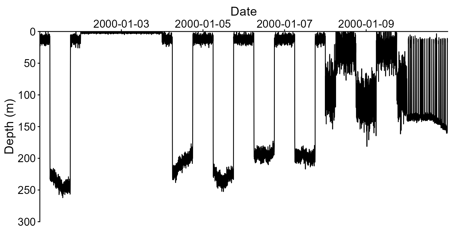

Depth record of the example tag over ten days, with depth increasing downwards from 0 to 300 metres. — The example tag’s depth record: ten days at one-minute sampling, made with `plot_TDR()`.

2. Wavelet analysis

create_wavelet() runs the continuous wavelet transform over a range of periods, from lower_period_mins up to upper_period_hours, with suboctaves periods for each doubling of period.

Lower period: The shortest cycle analysed. 5 minutes captures short dives, where the sampling interval allows; it must be at least twice the sampling interval. This example uses 30 minutes to keep it quick.
Upper period: The longest cycle analysed. 24 hours focuses on daily behaviour.
Sub-octaves: 12 gives periods that include 24, 12 and 6 hours exactly, with 12 periods between each.

Use the same settings for all tags you will cluster together.

wavelet <- create_wavelet(
  archive = archive_days,
  tag_ID = "data",
  lower_period_mins = 30,
  upper_period_hours = 24,
  suboctaves = 12,
  output = TRUE,
  output_folder = project,
  plot_wavelet = TRUE,
  interactive_mode = FALSE
)

With plot_wavelet = TRUE, the power spectrum is saved in the tag’s 2_Wavelet_Figures folder. Red shows strong oscillation at that period and time.

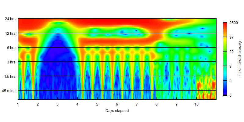
Wavelet power spectrum of the example tag: days elapsed along the bottom, period from 30 minutes to 24 hours up the side, with red showing strong power. — Wavelet power spectrum of the example tag, made with `create_wavelet()`. The strong band at 24 hours is the daily cycle; short-period power near day 10 comes from repeated dives.

Wavelets of long, high-frequency records can need a lot of memory: a year at 1-second sampling can need tens of gigabytes. Large, high-frequency records explains how to estimate this and how to reduce it with thin_archive().

3. Daily statistics

create_wavelet_stats() summarises the wavelet for each day and period: mean and variance of the amplitude, phase and power, and the mean squared power.

wave_stats <- create_wavelet_stats(wavelet, tag_ID = "data", output = TRUE, output_folder = project)
dim(wave_stats)
#> [1]  10 478

create_depth_stats() calculates daily statistics from the full-resolution depth record: mean, standard deviation, minimum and maximum depth, mean vertical speed, maximum descent and ascent speeds, skewness and kurtosis of depth, and the proportion of time near the surface.

With diel = TRUE it adds the differences between night and day in these statistics, standardised by each day’s maximum depth. Sunrise and sunset come from a GPS file with daily positions (columns date, lat and lon), or from fixed sunrise_time and sunset_time.

depth_stats <- create_depth_stats(
  archive = archive_days,
  tag_ID = "data",
  diel = TRUE,
  GPS = file.path(example_folder, "data", "GPS.csv"),
  sunset_type = "civil",
  output = TRUE,
  output_folder = project
)
names(depth_stats)
#>  [1] "date_only"          "depth.mean"         "depth.sd"
#>  [4] "depth.min"          "depth.max"          "mean.abs_vv"
#>  [7] "max.dsc_vv"         "max.asc_vv"         "skewness_depth"
#> [10] "kurtosis_depth"     "surface_proportion" "st_mean_diff"
#> [13] "st_sd_diff"         "st_range_diff"      "st_absVV_diff"
#> [16] "st_dscVV_diff"      "st_ascVV_diff"      "surf_prop_diff"

4. Principal component analysis

pca_data() collects the chosen wavelet statistics for the tags to analyse. Mean power, power variance and mean amplitude are the defaults: they capture the most variance in the fewest principal components.

pc_data <- pca_data(
  tag_vector = "data",
  data_folder = project,
  power_mean = TRUE,
  power_variance = TRUE,
  amplitude_mean = TRUE
)

Before choosing how many components to keep, look at the eigenvalues and the cumulative variance they explain. Asking for up to 50 components returns all of their eigenvalues.

all_pcs <- pca_results(pc_data, No_pcs = 50, plot_eigenvalues = FALSE, interactive_mode = FALSE)
round(head(all_pcs$eig, 8), 2)
#>        eigenvalue percentage of variance cumulative percentage of variance
#> comp 1     108.02                  52.95                             52.95
#> comp 2      55.82                  27.36                             80.31
#> comp 3      24.25                  11.89                             92.20
#> comp 4       8.77                   4.30                             96.50
#> comp 5       3.95                   1.94                             98.43
#> comp 6       1.80                   0.88                             99.32
#> comp 7       0.87                   0.43                             99.74
#> comp 8       0.32                   0.16                             99.90

Common choices are the components with eigenvalues of 1 or more, or enough components to explain at least 70% of the variance. Here three components explain over 90%.

pc_results <- pca_results(pc_data, No_pcs = 3, plot_eigenvalues = FALSE, interactive_mode = FALSE)
pc_scores <- pca_scores(pc_results, plot_loadings = FALSE)

combine_data() joins each day’s principal component scores with its depth statistics, ready for clustering.

kmeans_data <- combine_data(tag_vector = "data", data_folder = project, pc_scores = pc_scores)
dim(kmeans_data)
#> [1] 10 22

5. Choose the number of clusters and cluster the days

select_k() runs k-means for each number of clusters up to Max.k, and plots the within-cluster sum of squares (A, the “elbow” plot) and the mean silhouette width (B). Look for a number near the elbow, where more clusters stop reducing the sum of squares by much, and where the silhouette width is high. K-means starts from random cluster centres, so set a seed for reproducible results.

set.seed(123)
select_k(kmeans_data, Max.k = 8, v_line = 4)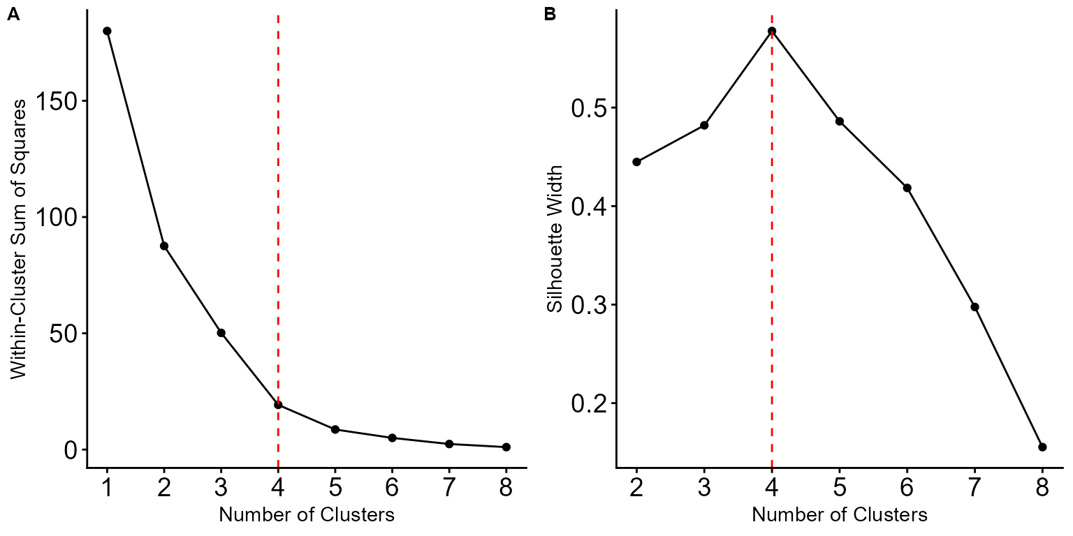

Two plots against the number of clusters: within-cluster sum of squares falling steeply until four clusters, and silhouette width peaking at four clusters, with a dashed line at four. — Choosing k with `select_k()`: the elbow (A) and the highest silhouette width (B) both point to four clusters.

k_clustering() assigns each day to one of k clusters. With output = TRUE it also saves a 3D plot of the first three principal components and figures of each cluster’s mean variable values.

set.seed(123)
kmeans_result <- k_clustering(kmeans_data, k = 4, nstart = 50, output = FALSE)
table(Cluster = kmeans_result$cluster)
#> Cluster
#> 1 2 3 4
#> 2 1 2 5

With only ten days, these clusters are just for illustration: real analyses need many more days for meaningful clusters.

6. Plot the results

plot_cluster_TDR() plots a tag’s depth record with each day coloured by its cluster.

plot_cluster_TDR(
  tag_ID = "data",
  data_folder = project,
  kmeans_result = kmeans_result,
  minmax_bins = 2000,
  Y_lim = c(0, 300, 50),
  date_breaks = "2 day"
)

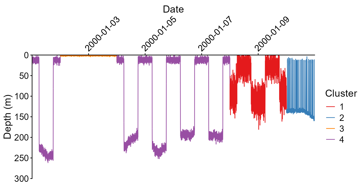
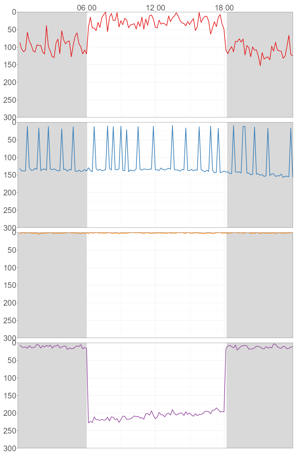
The example tag’s depth record as one continuous line, with each day coloured by its behaviour cluster, one to four. — The depth record coloured by cluster, made with `plot_cluster_TDR()`. The record stays one continuous line; only the colour changes from day to day.

plot_clusters() plots the most typical days of each cluster: those closest to the cluster’s centre. With diel_shade = TRUE, night is shaded grey. It saves one figure per cluster, and combined figures, in the tag’s 6_Cluster-plots folder.

plots <- plot_clusters(
  tag_vector = "data",
  data_folder = project,
  kmeans_result = kmeans_result,
  No_days = 1,
  Y_lim = c(0, 300, 50),
  diel_shade = TRUE,
  dpi = 72,
  output = TRUE,
  output_folder = project
)

The most typical day of each of the four clusters, stacked from cluster 1 at the top to cluster 4 at the bottom, with night shaded grey. — The most typical day of each cluster, 1 to 4 from the top, with night shaded. Cluster 1 stays shallow by day and goes deeper at night; cluster 2 dives repeatedly from about 140 m to the surface; cluster 3 stays at the surface; cluster 4 is near the surface at night and around 200 m by day, the pattern of diel vertical migration.

Analysing several tags together

Clustering several tags together finds behaviours shared between individuals. Run steps 1 to 3 for each tag with the same project folder and wavelet settings, then pass all the tag IDs to pca_data() and combine_data():

tags <- c("tag_A", "tag_B", "tag_C")
pc_data <- pca_data(tag_vector = tags, data_folder = project, output = TRUE, output_folder = project)
# ... pca_results() and pca_scores() as above ...
kmeans_data <- combine_data(tag_vector = tags, data_folder = project, pc_scores = pc_scores)

Results for several tags are saved in the project’s Combined_tags folder, and plot_clusters() takes the same tag_vector. Tags analysed together should have the same wavelet settings, and ideally the same sampling interval (see thin_archive()).

Function reference

import_tag_data(): Load a time-depth series from a CSV file, and crop it to the deployment and to whole local days.
plot_TDR(): Plot the time-depth record.
thin_archive(): Thin a depth record to a longer sampling interval by block-averaging, before the wavelet. Development version.
create_wavelet(): Run the continuous wavelet transform and plot the wavelet power spectrum.
create_wavelet_stats(): Summarise the wavelet for each day and period.
create_depth_stats(): Calculate daily depth statistics and, optionally, diel (day and night) statistics.
pca_data(): Collect the chosen wavelet statistics for principal component analysis.
pca_results(): Run the principal component analysis and choose the number of components.
pca_scores(): Extract each day’s principal component scores.
combine_data(): Join the principal component scores with the depth statistics, ready for clustering.
select_k(): Plot the elbow and silhouette widths to help choose the number of clusters.
k_clustering(): Cluster the days with k-means.
plot_cluster_TDR(): Plot a tag’s depth record with each day coloured by its cluster.
plot_clusters(): Plot the days closest to the centre of each cluster.
run_app(): Open the point-and-click app. Development version.

Full details of every argument are in the package help, for example ?create_wavelet, and in the online function reference.

Citing FishDiveR

If you use FishDiveR in published work, please cite the methods paper. The full reference and a BibTeX entry are on the FishDiveR overview.

Stuck, or want a second pair of eyes?

I created and maintain the package. Please report problems on GitHub, see analysis services if you’d rather I ran the analysis for you, or email me.

[email protected]